{% extends "::base.html.twig" %}

{% block title %}{{ parent() }}about{% endblock %}

{% block header %}
{{ parent() }}
<link rel="stylesheet" href="{{ asset('mixstore/css/static/about.css') }}">
{% endblock %}

{% block content %}

<div id="maintext" class="row">

<div class="col-xs-12 borderbottom">

<h2>Origins</h2>

In the late 1990's, three researchers wrote some code in MATLAB to classify data using 
mixture models. Initially named XEM for "EM-algorithms on miXture models", 
it was quickly renamed into mixmod, and rewritten in C++ from 2001. 
Since then, mixmod has been extended in several directions including:
<ul>
	<li>supervised classification</li>
	<li>categorical data handling</li>
	<li>heterogeneous data handling</li>
</ul>
...and the code is constantly evolving. {# still in constant evolution #} 
More details can be found on the <a href="http://www.mixmod.org">dedicated website</a>.

There exist now many packages related to mixture models, each of them specialized in 
some domain. Although mixmod can (arguably) be considered as one of the first of its kind, 
it would be rather arbitrary to give him a central position. 
That is why mixmod is "only" part of the mix-store.

{# (mixmod permet de faire + de choses : renvoyer au site web + doc...) #}

<h2>Summary</h2>

Mixstore is a website gathering libraries dedicated to data modeling as 
a mixture of probabilistic components. The computed mixture can be used 
for various purposes including
<ul>
	<li>density estimation</li>
	<li>clustering (unsupervised classification)</li>
	<li>(supervised) classification</li>
	<li>regression, ...</li>
</ul>

<h2>Example</h2>

<p>
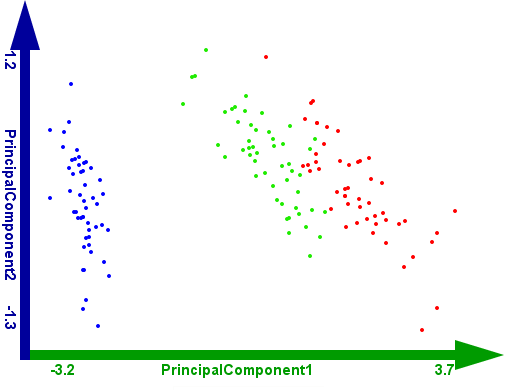
To start using any of the softwares present in the store, we need a dataset. 
We choose here an old classic: the Iris dataset introduced by Ronald Fisher in 1936. 
Despite its classicity this dataset is not so easy to analyze, as we will see in the following. 
</p>

<p>
The <a href="http://en.wikipedia.org/wiki/Iris_flower_data_set">Iris dataset</a> 
contains 150 rows, each of them composed of 4 continuous attributes which 
corresponds to some flowers measurements. 3 species are equally represented : (Iris) 
Setosa, Versicolor and Virginica.
</p>

<p>
	<figure>
	<img src="{{ asset('mixstore/images/iris_pca.png') }}" alt="PCA components of iris dataset"/><br/>
	<caption>The two first PCA components of Iris dataset (image found 
	<a href="http://www.wanderinformatiker.at/unipages/general/img/iris_pca1.png">here</a>)</caption>
	</figure>
</p>

<p>
As the figure suggests the goal on this dataset is to discriminate Iris species. 
That is to say, our goal is to find a way to answer these questions: 
"are two given elements in the same group ?", "which group does a given element belongs to ?".
</p>

<p>
The mixstore packages take a more general approach: they (try to) learn the data generation 
process, and then deduce the groups compositions. Thus, the two above questions can easily 
be answered by using the mathematical formulas describing the classes.
Although this approach has several advantages (low sensitivity to outliers, likelihood 
to rank models...), finding the adequate model is challenging. 
We will not dive into such model selection details.
{# This is a more general and harder problem. #}
</p>

</div>

<div class="col-xs-12">

<p>
Density for 2 groups:
££f^{(2)}(x) = \pi_1^{(2)} g_1^{(2)}(x) + \pi_2^{(2)} g_2^{(2)}(x)££
where £g_i^{(2)} = (2 \pi)^{-d/2} \left| \Sigma_i^{(2)} \right|^{-1/2} \mbox{exp}\left( -\frac{1}{2} \, {}^T(x - \mu_i^{(2)}) (\Sigma_i^{(2)})^{-1} (x - \mu_i^{(2)}) \right)£.<br/>
£x = (x_1,x_2,x_3,x_4)£ with the following correspondances.
<ul>
	<li>£x_1£: sepal length;</li>
	<li>£x_2£: sepal width;</li>
	<li>£x_3£: petal length;</li>
	<li>£x_4£: petal width.</li>
</ul>
</p>

</div>

<div class="col-xs-12 col-sm-6">
\begin{align*}
\pi_1^{(2)} &= 0.33\\
\mu_1^{(2)} &= (5.01 3.43 1.46 0.25)\\
\Sigma_1^{(2)} &=
	\begin{pmatrix}
	0.15&0.13&0.02&0.01\\
	0.13&0.18&0.02&0.01\\
	0.02&0.02&0.03&0.01\\
	0.01&0.01&0.01&0.01
	\end{pmatrix}
\end{align*}
</div>

<div class="col-xs-12 col-sm-6">
\begin{align*}
\pi_2^{(2)} &= 0.67\\
\mu_2^{(2)} &= (6.26 2.87 4.91 1.68)\\
\Sigma_2^{(2)} &= 
	\begin{pmatrix}
	0.40&0.11&0.40&0.14\\
	0.11&0.11&0.12&0.07\\
	0.40&0.12&0.61&0.26\\
	0.14&0.07&0.26&0.17
	\end{pmatrix}
\end{align*}
</div>

<div class="col-xs-12 borderbottom">
Penalized log-likelihood (BIC): <b>-561.73</b>
</div>

<div class="col-xs-12">

<p>
Density for 3 groups:
££f^{(3)}(x) = \pi_1^{(3)} g_1^{(3)}(x) + \pi_2^{(3)} g_2^{(3)}(x) + \pi_3^{(3)} g_3^{(3)}(x)££
(Same parameterizations for cluster densities £g_i^{(3)}£).<br/>
</p>

</div>

<div class="col-xs-12 col-md-4">
\begin{align*}
\pi_1^{(3)} &= 0.33\\
\mu_1^{(3)} &= (5.01 3.43 1.46 0.25)\\
\Sigma_1^{(3)} &=
	\begin{pmatrix}
	0.13&0.11&0.02&0.01\\
	0.11&0.15&0.01&0.01\\
	0.02&0.01&0.03&0.01\\
	0.01&0.01&0.01&0.01
	\end{pmatrix}
\end{align*}
</div>

<div class="col-xs-12 col-md-4">
\begin{align*}
\pi_2^{(3)} &= 0.30\\
\mu_2^{(3)} &= (5.91 2.78 4.20 1.30)\\
\Sigma_2^{(3)} &= 
	\begin{pmatrix}
	0.23&0.08&0.15&0.04\\
	0.08&0.08&0.07&0.03\\
	0.15&0.07&0.17&0.05\\
	0.04&0.03&0.05&0.03
	\end{pmatrix}
\end{align*}
</div>

<div class="col-xs-12 col-md-4">
\begin{align*}
\pi_3^{(3)} &= 0.37\\
\mu_3^{(3)} &= (6.55 2.95 5.48 1.96)\\
\Sigma_3^{(3)} &= 
	\begin{pmatrix}
	0.43&0.11&0.33&0.07\\
	0.11&0.12&0.09&0.06\\
	0.33&0.09&0.36&0.09\\
	0.07&0.06&0.09&0.09
	\end{pmatrix}
\end{align*}
</div>

<div class="col-xs-12 borderbottom">
Penalized log-likelihood (BIC): <b>-562.55</b>
</div>

<div class="col-xs-12">

<p>
As initially stated, the dataset is difficult to cluster because although we know there are 
3 species, 2 of them are almost undinstinguishable. That is why log-likelihood values are very close. 
We usually consider that a method is good on Iris dataset when it finds 3 clusters, 
but 2 is also a correct answer.
</p>

</div>

</div>

{% endblock %}

{% block javascripts %}
{{ parent() }}
<script type="text/x-mathjax-config">
MathJax.Hub.Config({
	tex2jax: {
		inlineMath: [['£','£']],
		displayMath: [['££','££']],
		skipTags: ["script","noscript","style"]//,"textarea","pre","code"]
	}
});
</script>
<script src="http://cdn.mathjax.org/mathjax/latest/MathJax.js?config=TeX-AMS_HTML"></script>
{% endblock %}